Detect out of range outliers in sensor data

Introduction

The out_of_range() function uses Savitzky-Golay smoothing (SG) - sg() to estimate the main trend of the data:

The algorithm carries out two iterations to determine the trend and detect extreme outliers.

The outlier detection is based on the studentized residuals and the Bonferroni Correction. The residuals between the original data and the estimated trend are studentized and the Bonferroni Correction is used to identify potential outliers.

Note that the Out of Range algorithm is designed to be used with non-linear, non-stationary sensor data. Therefore, lets start by generating a synthetic signal with those characteristics. We will use some of the signal generator functions in InDSL. We also need a few additional InDSL helper functions and algorithms to demonstrate how the outlier detection works step by step.

import matplotlib.pyplot as plt
import numpy as np
import pandas as pd

from scipy.stats import t as student_dist

from datasets.data.synthetic_industrial_data import non_linear_non_stationary_signal
from indsl.data_quality.outliers import (
    _calculate_hat_diagonal,
    _calculate_residuals_and_normalize_them,
    _split_timeseries_into_time_and_value_arrays,
    out_of_range,
)
from indsl.resample import reindex
from indsl.smooth import sg

Non-linear, non-stationary synthetic signal

We’ll use a pre-defined test data set with a non-linear, non-stationary time series with “industrial” characteristics. This data set is a time series composed of 3 oscillatory components, 2 nonlinear trends, sensor linear drift (small decrease over time) and white noise. The signal has non-uniform time stamps, a fraction (35%) of the data is randomly removed to generate data gaps. The data gaps and white noise are inserted with a constant seed to have a reproducible behavior of the algorithm. The functions used to generate this signal are also part of InDSL: insert_data_gaps(), line(), perturb_timestamp(), sine_wave(), and white_noise().

seed_array = [10, 1975, 2000, 6000, 1, 89756]
seed = seed_array[4]
data = non_linear_non_stationary_signal(seed=seed)


# A simple function to style and annotate the figures.
def style_and_annotate_figure(
    ax,
    text,
    x_pos=0.50,
    y_pos=0.9,
    fsize=12,
    fsize_annotation=18,
    title_fsize=14,
    ylimits=[-3005, 8000],
    title_txt=None,
):
    ax.text(
        x_pos, y_pos, text, transform=ax.transAxes, ha="center", va="center", fontsize=fsize_annotation, color="dimgrey"
    )
    ax.legend(fontsize=fsize, loc=4)
    ax.tick_params(axis="both", which="major", labelsize=fsize)
    ax.tick_params(axis="both", which="minor", labelsize=fsize)
    ax.tick_params(axis="x", rotation=45)
    ax.set_title(title_txt, fontsize=title_fsize)
    ax.grid()
    ax.set_ylim(ylimits)

Insert extreme outliers

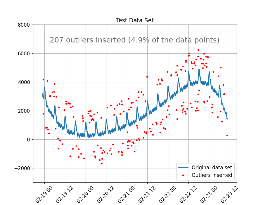
This algorithm was tested with outliers generated at different locations. Five percent (5%) of the data points at random locations were replaced by outliers. To do so we used |Numpy's| random generator with different seeds. Feel free to use one of the 5 seeds below. The algorithm will work with 100% precision for these conditions and parameters used in the example. Or use another seed to generate a different signal and further test the limits of the algorithm.

data = data.dropna()

rng = np.random.default_rng(seed)
outlier_fraction = 0.05  # Fraction of the signal that will be replaced by outliers
num_outliers = round(len(data) * outlier_fraction)
locations = np.unique(rng.integers(low=0, high=len(data), size=num_outliers))
direction = rng.choice([1, -1], size=len(locations))
outliers = data.iloc[locations] + data.mean() * rng.uniform(0.5, 1, len(locations)) * direction

data_w_outliers = data.copy()
data_w_outliers[locations] = outliers

Initial conditions: test data set

The figure below shows the original data set and the outliers inserted. We took care to give the outliers random values, both far and close to the main trend. But far enough for these to be categorized as an extreme deviation from the expected behavior of the data.

fig_size = (9, 7)
fig, ax = plt.subplots(figsize=fig_size)
ax.plot(data, linewidth=2, label="Original data set")
ax.plot(outliers, "ro", markersize=3, label="Outliers inserted")
outliers_inserted = (
    f"{len(outliers)} outliers inserted ({round(100 * len(outliers) / len(data), 1)}% of the data points)"
)
style_and_annotate_figure(ax, text=outliers_inserted, title_txt="Test Data Set")

Initial iteration

1. Trend estimate

As mentioned before, we will use a SG smoother to estimate the trend. To demonstrate how the initial pass works, we’ll run the SG independently. The SG smoother requires a point-wise window length and a polynomial order. The bigger the window, more data used to estimate the local trend. With the polynomial order we influence how much we want the fit to follow the non-linear characteristics of the data (1, linear, >1 increasingly non-linear fit). In this case we will use a window of 20 data points and 3rd order polynomial fit.

# Estimate the trend using Savitzky-Golay smoother
tolerance = 0.08
trend_pass01 = sg(data_w_outliers, window_length=20, polyorder=3)

2. Studentized residuals and Bonferroni correction

Identifying potential outliers is done by comparing how much each data point deviates from the estimated main trend (i.e. the residuals). However, since in most cases little information about the data is readily available and extreme outliers are expected to be sparse and uncommon, the Student's-t distribution is well suited for the current task, where the sample size is small and the standard deviation is unknown. To demonstrate how the residuals are studentized, we use a helper function from InDSL. But these steps are integrated into the out_of_range() function. Finally, since we aim to identify extreme outliers, a simple t-test does not suffice. Hence the Bonferroni Correction. Furthermore, we use a relaxation factor for the Bonferroni factor estimated from the data to adjust the sensitivity of the correction. Again, the Bonferroni Correction is explicitly calculated here but it is integrated into the out_of_range() function.

# Statistical parameters
alpha = 0.05  # Significance level or probability of rejecting the null hypothesis when true.
bc_relaxation = 1 / 4  # Bonferroni relaxation coefficient.

x, y = _split_timeseries_into_time_and_value_arrays(data_w_outliers)
y_pred_pass01 = trend_pass01.to_numpy()
hat_diagonal = _calculate_hat_diagonal(x)

# Calculate degrees of freedom (n-p-1)
n = len(y)
dof = n - 3  # Using p = 2 for a model based on a single time series

# Calculate Bonferroni critical value and studentized residuals
bc = student_dist.ppf(1 - alpha / (2 * n), df=dof) * bc_relaxation
t_res = _calculate_residuals_and_normalize_them(dof, hat_diagonal, y, y_pred_pass01)

# Boolean mask where outliers are detected
mask = np.logical_and(t_res < bc, t_res > -bc)
filtered_ts_pass01 = pd.Series(y[mask], index=data.index[mask])  # Remove detected outliers from time series

outliers_pass01 = pd.Series(y[~mask], index=data.index[~mask])

3. Outliers detected with the initial pass

The figure below shows the results of the initial pass. The SG method does a good job at estimating the trend, except for a few periods in the data where a larger number of outliers are grouped together. This causes strong nonlinear behavior in the estimated trend, and as a consequence some data points are miss-identified as outliers. But overall, a good enough baseline.

fig2, ax2 = plt.subplots(figsize=fig_size)
ax2.plot(data_w_outliers, "--", color="orange", label="Data with outliers")
ax2.plot(trend_pass01, "k", linewidth=2, label="Savitzky-Golay trend")
ax2.plot(outliers_pass01, "wo", markersize=7, alpha=0.85, mew=2, markeredgecolor="green", label="Outliers detected")
ax2.plot(outliers, "ro", markersize=3, label="Outliers inserted")

text_outlier_res = (
    f"{len(outliers_pass01)} out of {len(outliers)} outliers detected "
    f"({round(100 * len(outliers_pass01) / len(outliers), 1)}%)"
)
style_and_annotate_figure(ax2, text=text_outlier_res, title_txt="First Iteration: Savitzky-Golay trend")

Last iteration

For the last iteration the outliers previously detected are removed and then use the SG method to estimate the main trend.

tolerance_pass02 = 0.01
trend_pass02 = sg(filtered_ts_pass01, window_length=20, polyorder=3)

# Filtering parameters
alpha_pass02 = 0.05
bc_relaxation_pass02 = 1 / 2
bc_pass02 = student_dist.ppf(1 - alpha_pass02 / (2 * n), df=dof) * bc_relaxation_pass02

y_pred_pass02 = reindex(trend_pass02, data_w_outliers)
y_pred_pass02 = y_pred_pass02.to_numpy()
t_res_pass02 = _calculate_residuals_and_normalize_them(dof, hat_diagonal, y, y_pred_pass02)

# Boolean mask where outliers are detected
mask_pass02 = np.logical_and(t_res_pass02 < bc_pass02, t_res_pass02 > -bc_pass02)
filtered_ts_pass02 = pd.Series(y[mask_pass02], index=data.index[mask_pass02])

# Remove detected outliers from time series
outliers_pass02 = pd.Series(y[~mask_pass02], index=data.index[~mask_pass02])
# Run the InDSL function that carries out the entire analysis with the same parameters
indsl_outliers = out_of_range(data_w_outliers)

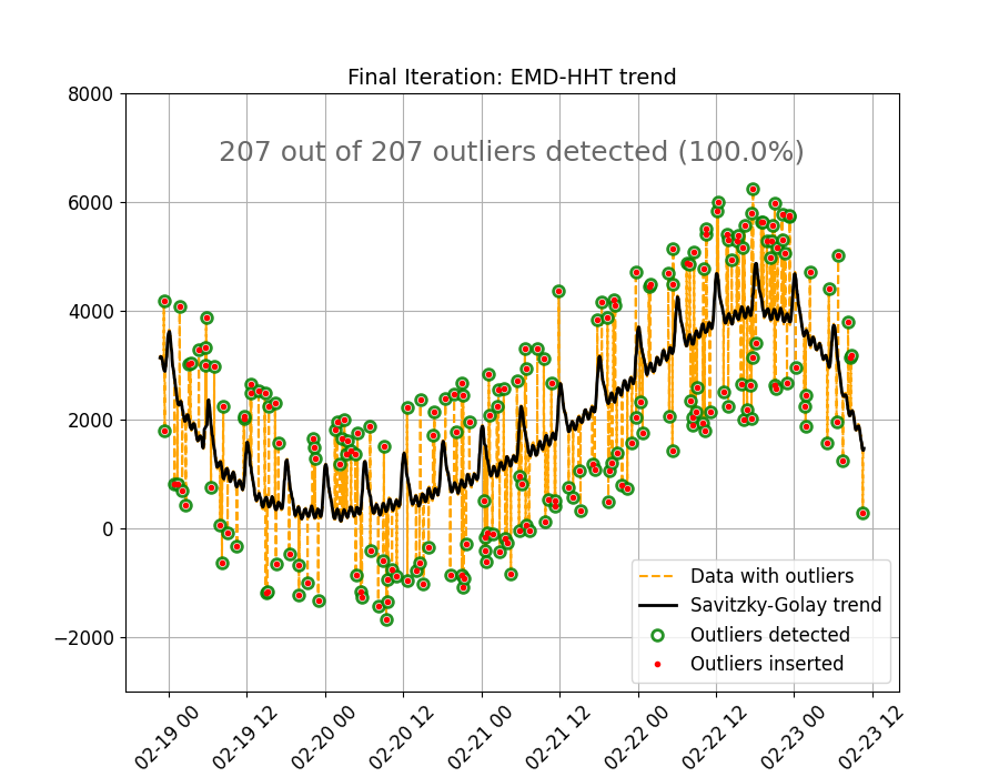
Results

The figure below shows the original data, the trend estimated using the SG method, the outliers artificially inserted, and the outliers detected by the full method (out_of_range()). A perfect performance is observed, all outliers are detected. This “perfect” performance will not always be the case but this function provides a very robust option for detecting and removing out of range or extreme outliers in non-linear, non-stationary sensor data.

# sphinx_gallery_thumbnail_number = 3
fig3, ax3 = plt.subplots(figsize=fig_size)

ax3.plot(data_w_outliers, "--", color="orange", label="Data with outliers")
ax3.plot(trend_pass02, "k", linewidth=2, label="Savitzky-Golay trend")
ax3.plot(
    indsl_outliers,
    "wo",
    markersize=7,
    alpha=0.85,
    mew=2,
    markeredgecolor="green",
    label="Outliers detected",
)
ax3.plot(outliers, "ro", markersize=3, label="Outliers inserted")

text_outlier_res = (
    f"{len(indsl_outliers)} out of {len(outliers)} outliers detected "
    f"({round(100 * len(indsl_outliers) / len(outliers), 1)}%)"
)

style_and_annotate_figure(ax3, text=text_outlier_res, title_txt="Final Iteration: EMD-HHT trend")
plt.show()