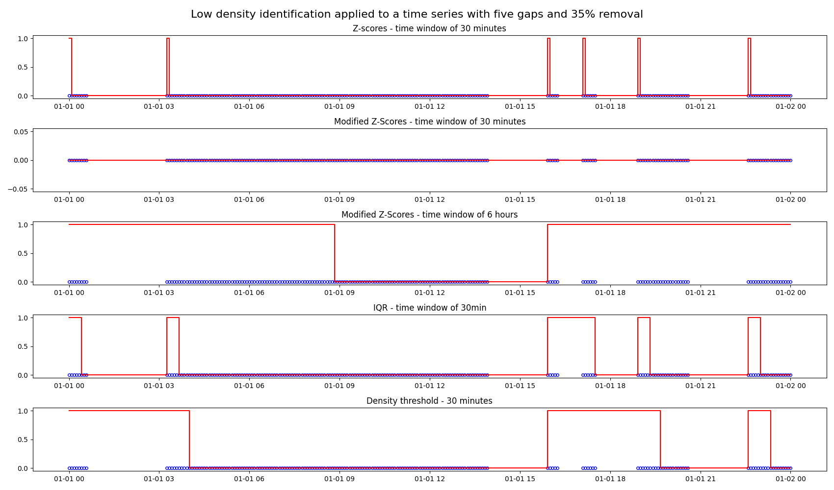
Identifying low density periods

Detecting density of data points in a time series is important for finding out if the expected number of data points during a certain time window such as per hour or per day have been received.

In this example, we apply four low-density identification methods to a time series. methods are:

1. Z-scores: Marks a period with low density if the number of data points is 3 standard deviations below the mean.

2. Modified Z-scores: A modified version of the Z-score method, which uses the median absolute deviation instead of the standard deviation.

3. Interquartile range (IQR): Uses IQR, a measure for the spread of the data, to identify low density periods.

4. Density threshold: Marks a period with low density if the number of data points are lower than the provided threshold.

In the plots below, we apply the four methods listed above to a time series ranging from 2022/01/01 to 2022/01/02 with sampling frequency of 5 minutes. In this time series, 35% of the data is removed by introducing five gaps at random locations. The plots show the different characteristics of the low density identification methods.

Low density identification using the modified Z-Score method has been plotted at two different time windows, one for 30 minutes and the other for 6 hours. The plot for 30-minute time window is a straight line because modified z-score method measures how much an outlier differs from a typical score based on the median.

import matplotlib.pyplot as plt
import pandas as pd

from indsl.data_quality.low_density_identification import (
    low_density_identification_iqr,
    low_density_identification_modified_z_scores,
    low_density_identification_threshold,
    low_density_identification_z_scores,
)
from indsl.signals.generator import insert_data_gaps, line


start = pd.Timestamp("2022/01/01")
end = pd.Timestamp("2022/01/02")

# Create a time series with four gaps of random location and size
remove = 0.35
data = line(start_date=start, end_date=end, slope=0, intercept=0, sample_freq=pd.Timedelta("5m"))
ts_mult_gaps = insert_data_gaps(data=data, fraction=remove, method="Multiple", num_gaps=5)

# Apply low density identification methods to time series
ts_low_density_z_scores = low_density_identification_z_scores(ts_mult_gaps, time_window=pd.Timedelta("30m"))
ts_low_density_modified_z_scores_time_window_30m = low_density_identification_modified_z_scores(
    ts_mult_gaps, time_window=pd.Timedelta("30m")
)
ts_low_density_modified_z_scores_time_window_6h = low_density_identification_modified_z_scores(
    ts_mult_gaps, time_window=pd.Timedelta("6h"), cutoff=1
)
ts_low_density_iqr = low_density_identification_iqr(ts_mult_gaps, time_window=pd.Timedelta("30m"))
ts_low_density_w_threshold = low_density_identification_threshold(ts_mult_gaps, time_window=pd.Timedelta("60m"))

fig, (ax1, ax2, ax3, ax4, ax5) = plt.subplots(5, 1, figsize=(17, 10))
ax1.plot(ts_mult_gaps, "bo", mec="b", markerfacecolor="None", markersize=4)
ax1.plot(ts_low_density_z_scores, "r-")

ax2.plot(ts_mult_gaps, "bo", mec="b", markerfacecolor="None", markersize=4)
ax2.plot(ts_low_density_modified_z_scores_time_window_30m, "r-")

ax3.plot(ts_mult_gaps, "bo", mec="b", markerfacecolor="None", markersize=4)
ax3.plot(ts_low_density_modified_z_scores_time_window_6h, "r-")


ax4.plot(ts_mult_gaps, "bo", mec="b", markerfacecolor="None", markersize=4)
ax4.plot(ts_low_density_iqr, "r-")

ax5.plot(ts_mult_gaps, "bo", mec="b", markerfacecolor="None", markersize=4)
ax5.plot(ts_low_density_w_threshold, "r-")

ax1.set_title("Z-scores - time window of 30 minutes")
ax2.set_title("Modified Z-Scores - time window of 30 minutes")
ax3.set_title("Modified Z-Scores - time window of 6 hours")
ax4.set_title("IQR - time window of 30min")
ax5.set_title("Density threshold - 30 minutes")

fig.suptitle("Low density identification applied to a time series with five gaps and 35% removal", fontsize=16)
fig.tight_layout()

plt.show()