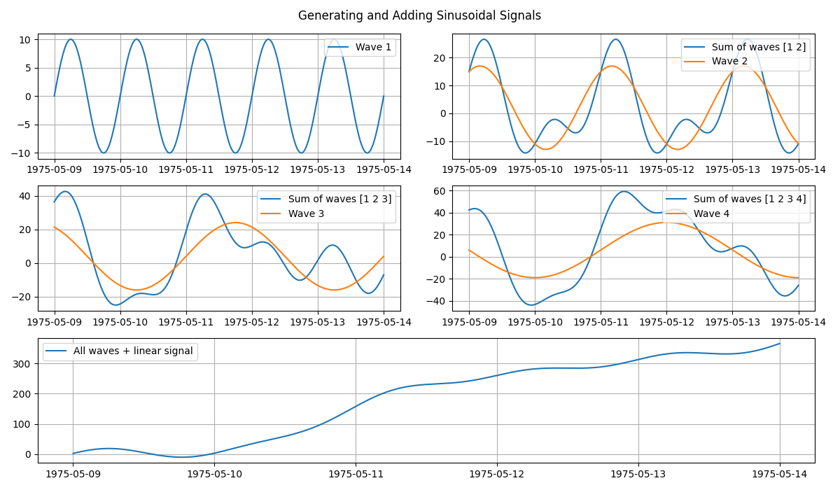
Wavy signal generation

Sinusoidal waves are very useful in signal generation. The sine wave equation can be used to generate a simple wave (wave 1 in the top left panel) or complex signals in a few steps. The figure below shows the generation of four different waves that are recursively added together to create an increasingly complex signal. And, combining it with other signals, such as sloping line, increases its functionality. The bottom panel of the figure shows all the waves plus a linearly increasing signal.

import matplotlib.pyplot as plt
import numpy as np
import pandas as pd

from indsl.signals.generator import line, sine_wave, wave_with_brownian_noise
from indsl.signals.noise import white_noise


# Define the signal and wave parameters
start = pd.Timestamp("1975-05-09")
end = pd.Timestamp("1975-05-14")
freq = pd.Timedelta("1 m")
w_period = [pd.Timedelta("1 D"), pd.Timedelta("2 D"), pd.Timedelta("3 D"), pd.Timedelta("4 D")]
w_mean = [0, 2, 4, 6]
w_amplitude = [10, 15, 20, 25]
w_phase = [0, np.pi * 1 / 3, np.pi * 2 / 3, np.pi]
color = ["b", "g", "r", "c"]

# Generate a plotting grid and recursively add all the waves
fig = plt.figure(tight_layout=True, figsize=[12, 7])
index = pd.date_range(start="1975-05-09", end="1975-05-14", freq="min")
all_waves = pd.Series(data=np.zeros(len(index)), index=index, dtype=float)
for item in range(len(w_period)):
    wave = sine_wave(
        start_date=start,
        end_date=end,
        sample_freq=freq,
        wave_period=w_period[item],
        wave_mean=w_mean[item],
        wave_amplitude=w_amplitude[item],
        wave_phase=w_phase[item],
    )
    all_waves = all_waves.add(wave)

    ax = plt.subplot(3, 2, item + 1)
    if item != 0:
        ax.plot(all_waves, label=f"Sum of waves {np.arange(item + 1) + 1}")
    ax.plot(wave, label=f"Wave {item + 1}")
    ax.legend(loc=1)
    ax.grid(True)

# Create a sloping line and add it to the sum of all the waves
linear_sig = line(
    start_date=start,
    end_date=end,
    sample_freq=freq,
    slope=1e-3,
    intercept=-40,
)

sloping_waves = all_waves + linear_sig
ax = plt.subplot(3, 2, (5, 6))
ax.plot(sloping_waves, label="All waves + linear signal")
ax.legend(loc=2)
ax.grid(True)
fig.suptitle("Generating and Adding Sinusoidal Signals")
plt.show()

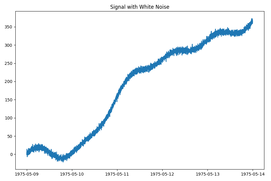
Add white noise

To make the final signal more realistic, let’s add white noise to it. We can use the indsl.signals.noise.white_noise() method. It will estimate the power (i.e. variance) of the signal and add white (random) noise to it, with a given signal-to-noise ratio (SNR).

fig = plt.figure(tight_layout=True, figsize=[9, 6])
plt.plot(white_noise(sloping_waves, snr_db=30))
plt.title("Signal with White Noise")
plt.show()

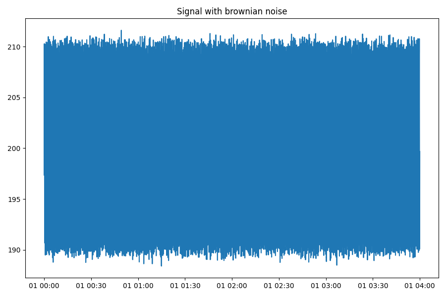
Add wave with brownian noise

We can use the indsl.signals.noise.wave_with_brownian_noise() method. It produces a sinusoidal signal with brownian noise.

fig = plt.figure(tight_layout=True, figsize=[9, 6])
plt.plot(wave_with_brownian_noise())
plt.title("Signal with brownian noise")
plt.show()