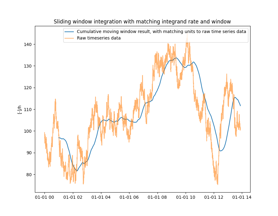
Sliding window integration

In this example a synthetic time series is generated with a certain skewness (to make it more interesting) and a use the sliding window integration with a integrand rate of 1 hour. In other words, carry out a sliding window integration of the data over 1 hour periods.

import matplotlib.pyplot as plt
import numpy as np
import pandas as pd

from indsl.ts_utils.numerical_calculus import sliding_window_integration


np.random.seed(1337)
datapoints = 5000
x = np.random.randn(datapoints)
y = np.zeros(len(x))
y[0] = x[0] + 100  # initial synthetic start
for i in range(1, len(x)):
    y[i] = y[i - 1] + (x[i] + 0.0025)  # and skew it upwards

series = pd.Series(y, index=pd.date_range(start="2000", periods=datapoints, freq="10s"))
result = sliding_window_integration(series, pd.Timedelta("1h"))

plt.figure(1, figsize=[9, 7])
plt.plot(result, label="Cumulative moving window result, with matching units to raw time series data")
plt.plot(series, alpha=0.6, label="Raw timeseries data")
plt.legend()
plt.ylabel("[-]/h")
plt.title("Sliding window integration with matching integrand rate and window")
_ = plt.show()