Trending with Empirical Mode Decomposition

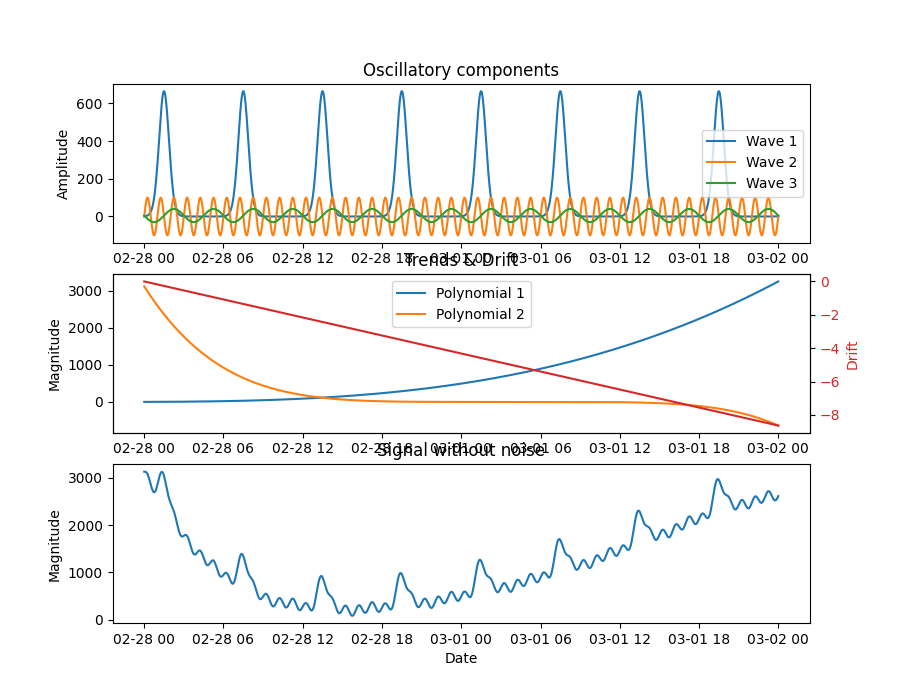
Example of trend extraction from non-linear, non-stationary signals using Empirical Mode Decomposition (EMD) and the Hilbert-Huang Transform. We generate a synthetic signal composed of:

• Three oscillatory signals of different but significant amplitudes

• Two polynomial functions or trends

• Data drift

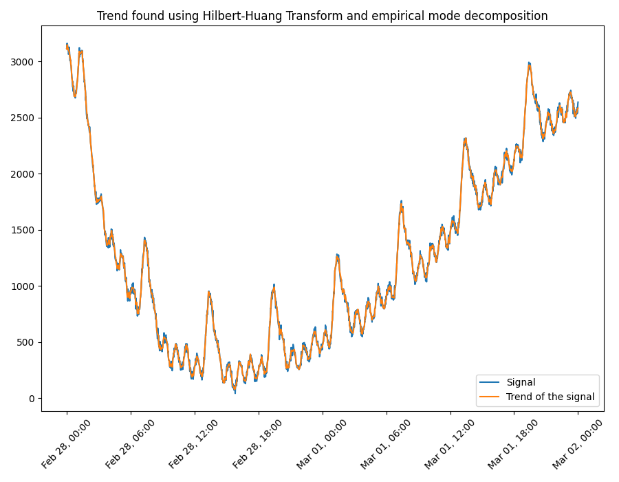
To make the case more realistic, from an industrial perspective, the timestamps are modified to make them nonuniform and 35% of the data points are randomly removed. Finally, Gaussian noise with a signal-to-noise ratio of 10 db is added to it.

The figure below shows each of the components of the synthetic signal (except for the Gaussian noise), the resulting synthetic signal and the trend obtained by means of Empirical Mode Decomposition and the Hilbert-Huang method implemented. It can be seen that the trend reflects the general signal behaviour. For example, the peak of the signal near Feb.28 13:00 is reflected in the estimated trend.

• 
• 

import matplotlib.pyplot as plt
import numpy as np
import pandas as pd

from matplotlib.dates import DateFormatter

from indsl.filter.trend import trend_extraction_hilbert_transform
from indsl.signals import insert_data_gaps, line, perturb_timestamp, sine_wave, white_noise


start_date = pd.Timestamp("2022-02-28")
end_date = pd.Timestamp("2022-03-02")

# Wave 1: Small amplitude, long wave period
wave01 = sine_wave(
    start_date=start_date,
    end_date=end_date,
    sample_freq=pd.Timedelta("1m"),
    wave_period=pd.Timedelta("6h"),
    wave_mean=0,
    wave_amplitude=6.5,
    wave_phase=0,
)
wave01 = np.exp(wave01)

# Wave 2: Large amplitude, short wave period
wave02 = sine_wave(
    start_date=start_date,
    end_date=end_date,
    sample_freq=pd.Timedelta("1m"),
    wave_period=pd.Timedelta("1h"),
    wave_mean=0,
    wave_amplitude=100,
    wave_phase=0,
)

# Wave 3: Large amplitude, short wave period
wave03 = sine_wave(
    start_date=start_date,
    end_date=end_date,
    sample_freq=pd.Timedelta("1m"),
    wave_period=pd.Timedelta("3h"),
    wave_mean=5,
    wave_amplitude=35,
    wave_phase=np.pi,
)

# Trends
trend_01 = (
    line(start_date=start_date, end_date=end_date, sample_freq=pd.Timedelta("1m"), slope=0.00008, intercept=1) ** 3
)

trend_02 = (
    line(start_date=start_date, end_date=end_date, sample_freq=pd.Timedelta("1m"), slope=-0.00005, intercept=5) ** 5
)

drift = line(start_date=start_date, end_date=end_date, sample_freq=pd.Timedelta("1m"), slope=0.00005, intercept=0)

signal = wave01 + wave02 + wave03 + trend_01 + trend_02 - drift
signal_w_noise = perturb_timestamp(white_noise(signal, snr_db=30))
signal_to_detrend = insert_data_gaps(signal_w_noise, method="Random", fraction=0.35)

trend = trend_extraction_hilbert_transform(signal_to_detrend)

fig, ax = plt.subplots(3, 1, figsize=[9, 7])

ax[0].plot(wave01, label="Wave 1")
ax[0].plot(wave02, label="Wave 2")
ax[0].plot(wave03, label="Wave 3")
ax[0].set_title("Oscillatory components")
ax[0].set_ylabel("Amplitude")
ax[0].legend()

ax[1].plot(trend_01, label="Polynomial 1")
ax[1].plot(trend_02, label="Polynomial 2")
ax[1].set_title("Trends & Drift")
ax[1].set_ylabel("Magnitude")
ax[1].legend()

color = "tab:red"
ax2 = ax[1].twinx()
ax2.plot(-drift, color=color)
ax2.set_ylabel("Drift", color=color)
ax2.tick_params(axis="y", labelcolor=color)

ax[2].plot(signal, label="Signal without noise")
ax[2].set_title("Signal without noise")
ax[2].set_ylabel("Magnitude")
ax[2].set_xlabel("Date")
plt.show()

# sphinx_gallery_thumbnail_number = 2
fig2, axs = plt.subplots(figsize=[9, 7])

# original signal
axs.plot(signal_to_detrend, label="Signal")

# Trend extracted from the signal
axs.plot(trend, label="Trend of the signal")

axs.set_title("Trend found using Hilbert-Huang Transform and empirical mode decomposition")

# Formatting x axis
# myFmt = DateFormatter("%b %d, %H:%M")
# axs.xaxis.set_major_formatter(myFmt)
axs.xaxis.set_major_formatter(DateFormatter("%b %d, %H:%M"))
plt.setp(axs.get_xticklabels(), rotation=45)
#
axs.legend(loc="lower right")
plt.tight_layout()

plt.show()